Investigation 1 · An effect and a threshold
Change the point estimate and standard error of a constructed mean difference. The nominal 95% normal interval is a simple illustration; it is not a substitute for the chapter's small-sample t procedures.
The target is a reduction, so a difference at or below the negative threshold is favourable. Selection, assignment, measurement and missingness must be reviewed separately.
Investigation 2 · The search itself matters
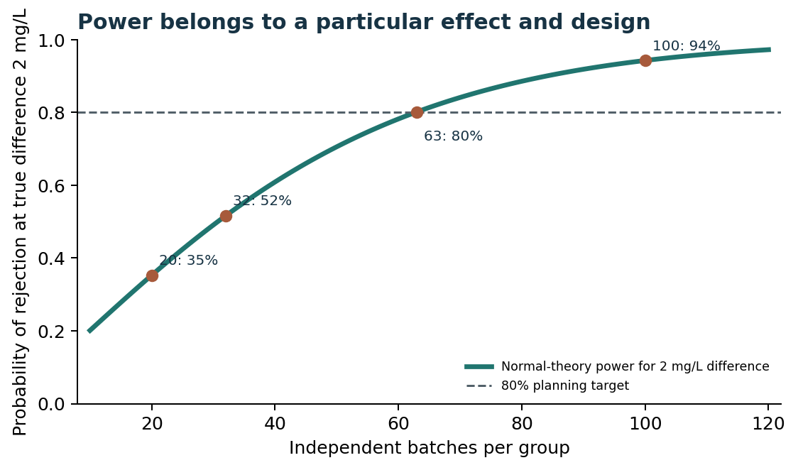
Under the special model that all nulls are true and tests are independent, see how the probability of at least one false rejection changes when more claims are screened at the same nominal level.
The simple independent-test formula changes with dependence and true effects. Bonferroni controls a different error quantity and can be conservative.
Read the observations
Download executed Python cases · Read draft exercise solutions
Report the evidence
- Name the target, eligible population and unit of assignment or observation.
- State the outcome and meaningful effect before selecting a test.
- Show the estimate and uncertainty in natural units.
- Explain the p-value only under its null and design.
- List missing data, measurement changes, multiple looks and subgroup searches.
Inspect the work.
Read the programs, run them in your own environment, and compare the results. The captured output records the chapter’s checked practical run; changing an input may change its answer.
Python testing_lab.py
"""Constructed Chapter 9 cases. Python 3 + SciPy; no external data."""

from math import comb, sqrt
from statistics import mean, variance

from scipy.stats import f, t, chi2


one = [-1, 0, 1, 2, 2, 2]
one_mean = mean(one)
one_var = variance(one)
one_se = sqrt(one_var / len(one))
one_t = one_mean / one_se
one_half = t.ppf(.975, len(one) - 1) * one_se
print(f"One sample: mean={one_mean:.6f}, variance={one_var:.6f}, SE={one_se:.6f}, t={one_t:.6f}, p={2*t.sf(abs(one_t),5):.6f}, CI=[{one_mean-one_half:.6f},{one_mean+one_half:.6f}]")

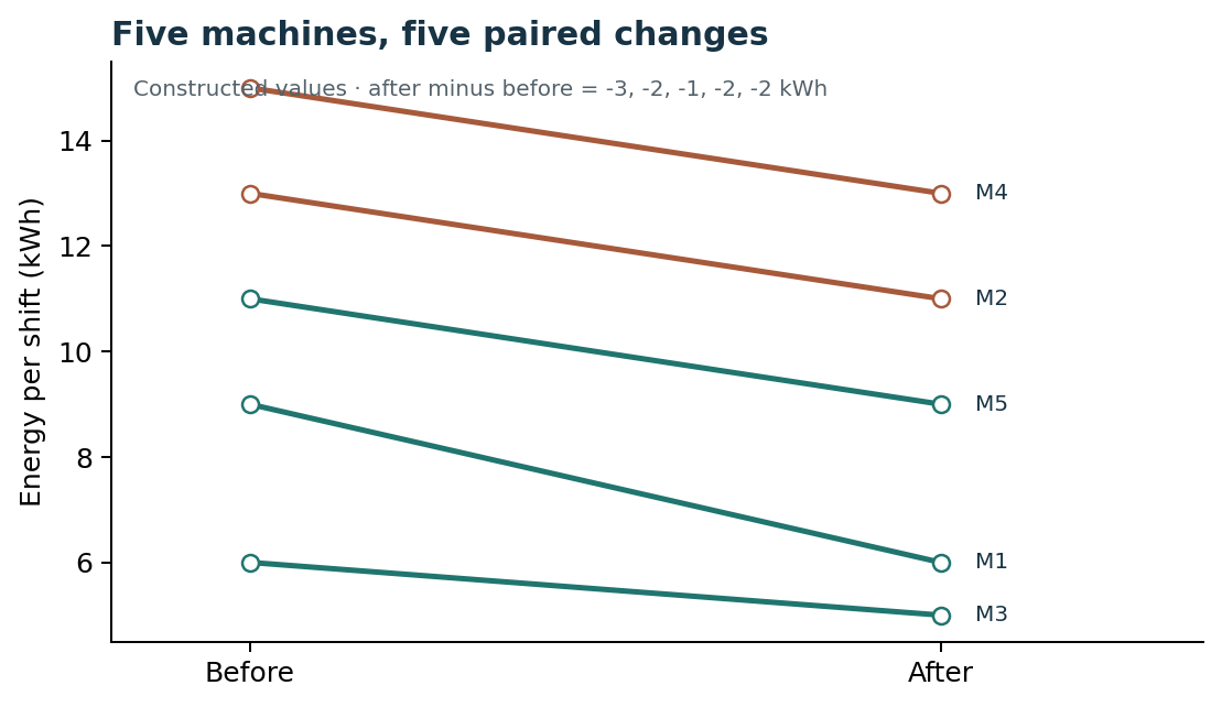
paired = [-3, -2, -1, -2, -2]
paired_mean = mean(paired)
paired_var = variance(paired)
paired_se = sqrt(paired_var / len(paired))
paired_t = paired_mean / paired_se
paired_half = t.ppf(.975, 4) * paired_se
print(f"Paired: mean={paired_mean:.6f}, variance={paired_var:.6f}, SE={paired_se:.6f}, t={paired_t:.6f}, p={2*t.sf(abs(paired_t),4):.6f}, CI=[{paired_mean-paired_half:.6f},{paired_mean+paired_half:.6f}]")

a, b = [4, 5, 6, 5], [5, 7, 9, 7]
diff = mean(b) - mean(a)
se = sqrt(variance(a)/len(a) + variance(b)/len(b))
v1, v2 = variance(a)/len(a), variance(b)/len(b)
df = (v1+v2)**2/(v1*v1/(len(a)-1)+v2*v2/(len(b)-1))
welch_t = diff / se
welch_half = t.ppf(.975,df)*se
print(f"Welch: difference={diff:.6f}, SE={se:.6f}, df={df:.6f}, t={welch_t:.6f}, p={2*t.sf(abs(welch_t),df):.6f}, CI=[{diff-welch_half:.6f},{diff+welch_half:.6f}]")

groups = [[3,4,5],[5,6,7],[7,8,9]]
grand = mean(x for g in groups for x in g)
ss_between = sum(len(g)*(mean(g)-grand)**2 for g in groups)
ss_within = sum(sum((x-mean(g))**2 for x in g) for g in groups)
f_stat = (ss_between/2)/(ss_within/6)
print(f"ANOVA: SSB={ss_between:.6f}, SSW={ss_within:.6f}, F={f_stat:.6f}, df=(2,6), p={f.sf(f_stat,2,6):.6f}")

observed = [[12,8],[8,12]]
row = [sum(r) for r in observed]
col = [sum(observed[i][j] for i in range(2)) for j in range(2)]
expected = [[row[i]*col[j]/sum(row) for j in range(2)] for i in range(2)]
chi = sum((observed[i][j]-expected[i][j])**2/expected[i][j] for i in range(2) for j in range(2))
print(f"Chi-square: expected={expected}, chi2={chi:.6f}, df=1, p={chi2.sf(chi,1):.6f}, risk_difference={12/20-8/20:.6f}")
print(f"Multiplicity: 20 independent true nulls, P(at least one p<.05)={1-.95**20:.6f}")
print(f"Randomisation: 8 units, 4 treated -> {comb(8,4)} assignments; hypothetical 4/70={4/70:.6f}")

assert abs(one_t-1.9364916731)<1e-8
assert abs(paired_t+sqrt(40))<1e-8
assert abs(se-sqrt(5/6))<1e-12
assert (ss_between,ss_within,f_stat)==(24,6,12)
assert chi==1.6
Output Checked chapter run
One sample: mean=1.000000, variance=1.600000, SE=0.516398, t=1.936492, p=0.110567, CI=[-0.327443,2.327443]
Paired: mean=-2.000000, variance=0.500000, SE=0.316228, t=-6.324555, p=0.003198, CI=[-2.877989,-1.122011]
Welch: difference=2.000000, SE=0.912871, df=4.411765, t=2.190890, p=0.087253, CI=[-0.443914,4.443914]
ANOVA: SSB=24.000000, SSW=6.000000, F=12.000000, df=(2,6), p=0.008000
Chi-square: expected=[[10.0, 10.0], [10.0, 10.0]], chi2=1.600000, df=1, p=0.205903, risk_difference=0.200000
Multiplicity: 20 independent true nulls, P(at least one p<.05)=0.641514
Randomisation: 8 units, 4 treated -> 70 assignments; hypothetical 4/70=0.057143