Investigation 1 · A binomial interval
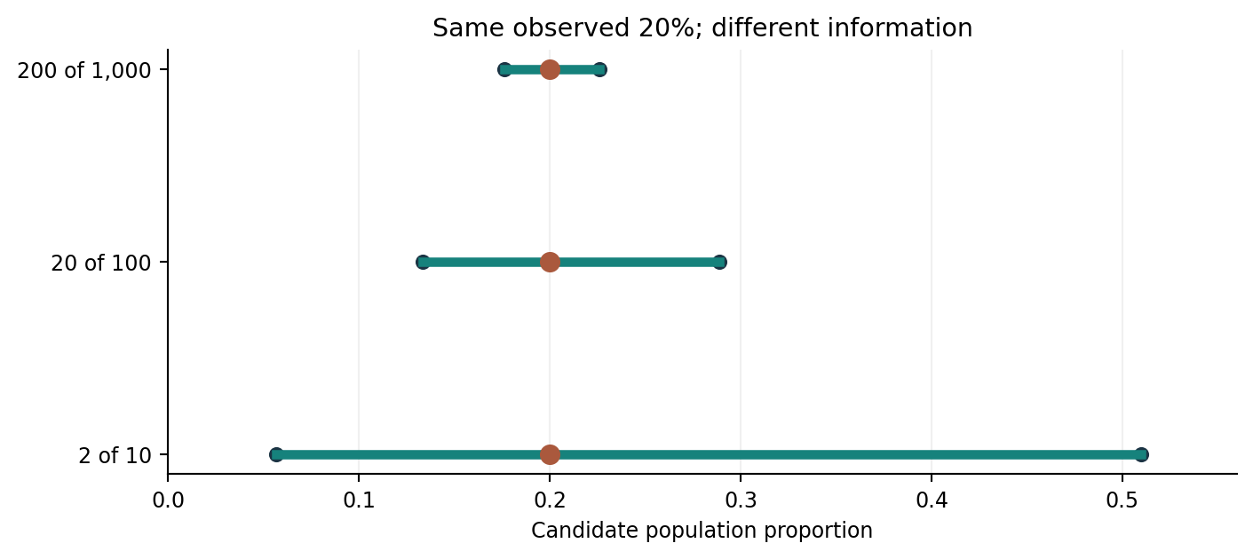
Enter successes and total eligible observations for an independent-binomial teaching model. Compare a simple symmetric interval with the Wilson score interval.
Observed fraction
Wilson nominal 95% interval
Simple symmetric interval
The interval only addresses uncertainty represented by the independent-binomial model.
Investigation 2 · Related rows
Try an equal-cluster planning approximation. It shows how records from the same source may carry less independent information than their row count suggests.
Design-effect approximation
Independent-equivalent rows (rough)
Real variance analysis must use the actual design and target; this single number is not a universal correction.
Read the evidence
Before writing the conclusion
- Name the target population and the sampling frame.
- Show how each observation could enter and how it was measured.
- State which variation the interval represents and what it omits.
- Compare the estimate and range with a decision threshold.
- Keep selection and measurement limitations beside the result.
Inspect the work.
Read the programs, run them in your own environment, and compare the results. The captured output records the chapter’s checked practical run; changing an input may change its answer.
Python inference_lab.py
"""Reproducible teaching checks for Chapter 8. No observed real-world data."""
from itertools import product
from math import sqrt
import numpy as np

def wilson(x,n,z=1.959963984540054):
 p=x/n;den=1+z*z/n;c=(p+z*z/(2*n))/den;h=z/den*sqrt(p*(1-p)/n+z*z/(4*n*n));return c-h,c+h
for x,n in ((2,10),(20,100),(200,1000)):
 lo,hi=wilson(x,n);print(f'Wilson {x}/{n}: [{lo:.6f}, {hi:.6f}]')
assert all(abs(a-b)<1e-6 for a,b in zip(wilson(2,10),(.056682151454375246,.5098375284633583)))
small=[0,1];vals=[sum(v)/4 for v in product(small,repeat=4)]
assert len(vals)==16 and abs(np.mean(vals)-.5)<1e-12 and abs(np.var(vals)-.0625)<1e-12
print('Exact n=4 Bernoulli sampling distribution: mean %.2f, SE %.2f' % (np.mean(vals),sqrt(np.var(vals))))
assert abs(.8*.1+.2*.3-.14)<1e-12
var=.8**2*.1*.9/50+.2**2*.3*.7/50
assert abs(var-.00132)<1e-12
print('Stratified estimate %.2f; illustrative SE %.6f' % (.14,sqrt(var)))
orig=[2,3,10];boots=[sum(v)/3 for v in product(orig,repeat=3)]
meds=[sorted(v)[1] for v in product(orig,repeat=3)]
assert len(boots)==27 and abs(np.var(boots)-38/9)<1e-12
assert [meds.count(v) for v in (2,3,10)]==[7,13,7]
print('Enumerated bootstrap means: SE %.6f; median counts 7/13/7' % sqrt(np.var(boots)))
assert abs(sqrt(.95*.05/10000)-.00217944947)<1e-8
print('Monte Carlo SE near 95%% / 10000: %.6f' % sqrt(.95*.05/10000))
rng=np.random.default_rng(20261115)
for p,n in ((.2,20),(.02,20),(.5,20),(.2,200)):
 k=rng.binomial(n,p,size=10000);ph=k/n
 wald_lo=ph-1.96*np.sqrt(ph*(1-ph)/n);wald_hi=ph+1.96*np.sqrt(ph*(1-ph)/n)
 den=1+1.96**2/n;c=(ph+1.96**2/(2*n))/den;h=1.96/den*np.sqrt(ph*(1-ph)/n+1.96**2/(4*n*n))
 wc=np.mean((c-h<=p)&(p<=c+h));ac=np.mean((wald_lo<=p)&(p<=wald_hi))
 print(f'Coverage p={p:.2f} n={n}: Wald {ac:.4f}, Wilson {wc:.4f} (10000 seeded runs)')
print('All assertions passed.')
Output Checked chapter run
Wilson 2/10: [0.056682, 0.509838]
Wilson 20/100: [0.133367, 0.288829]
Wilson 200/1000: [0.176377, 0.225919]
Exact n=4 Bernoulli sampling distribution: mean 0.50, SE 0.25
Stratified estimate 0.14; illustrative SE 0.036332
Enumerated bootstrap means: SE 2.054805; median counts 7/13/7
Monte Carlo SE near 95% / 10000: 0.002179
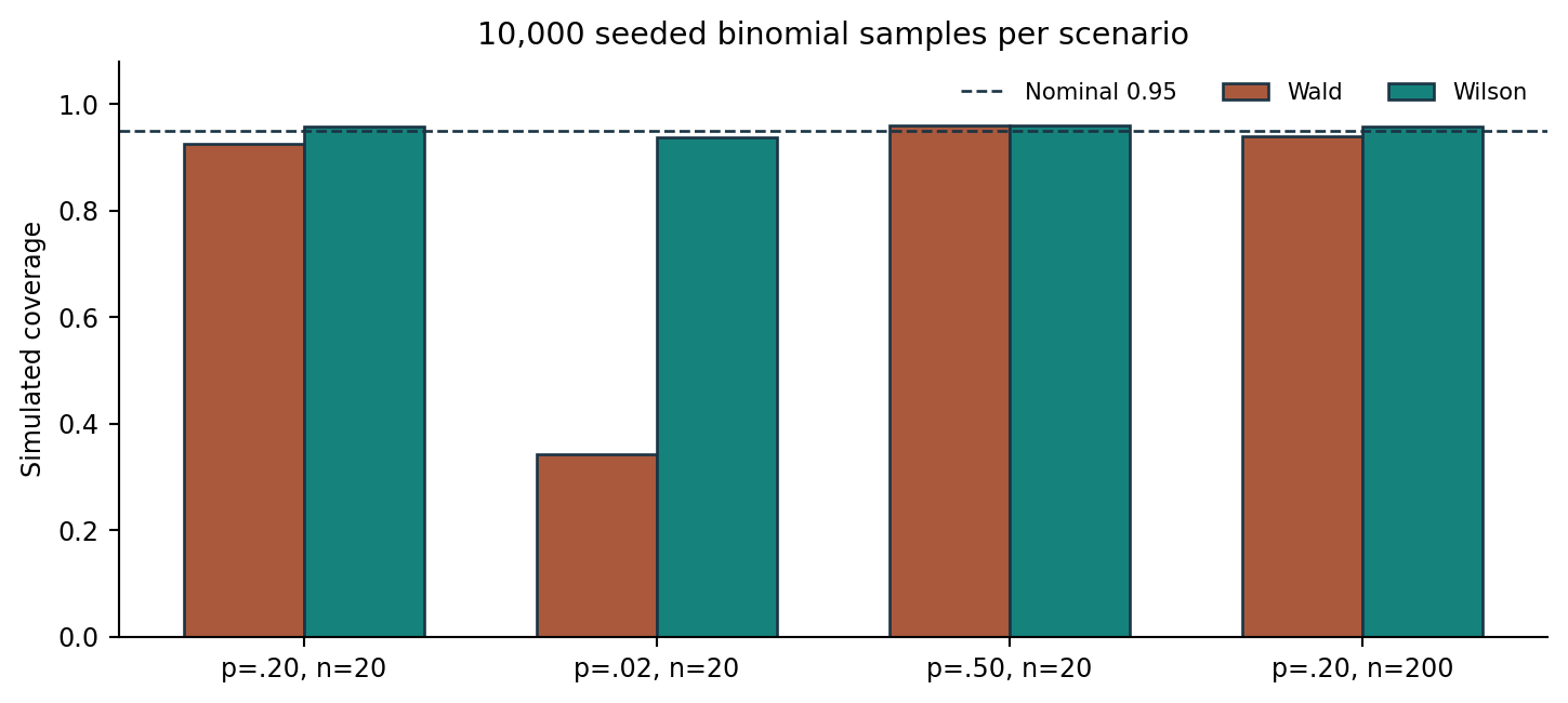
Coverage p=0.20 n=20: Wald 0.9249, Wilson 0.9571 (10000 seeded runs)
Coverage p=0.02 n=20: Wald 0.3420, Wilson 0.9379 (10000 seeded runs)
Coverage p=0.50 n=20: Wald 0.9588, Wilson 0.9588 (10000 seeded runs)
Coverage p=0.20 n=200: Wald 0.9387, Wilson 0.9578 (10000 seeded runs)
All assertions passed.