Investigation 1 · Exact assignments
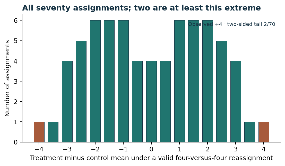
Eight fixed outcomes were assigned four-versus-four. Under the declared sharp null, there are seventy valid balanced assignments. Two have an absolute mean difference at least as large as the observed four units.
This is a probability over assignments under a sharp null, not a probability that the null is true. The classrooms example has a different assignment set.
Investigation 2 · Update a beta model
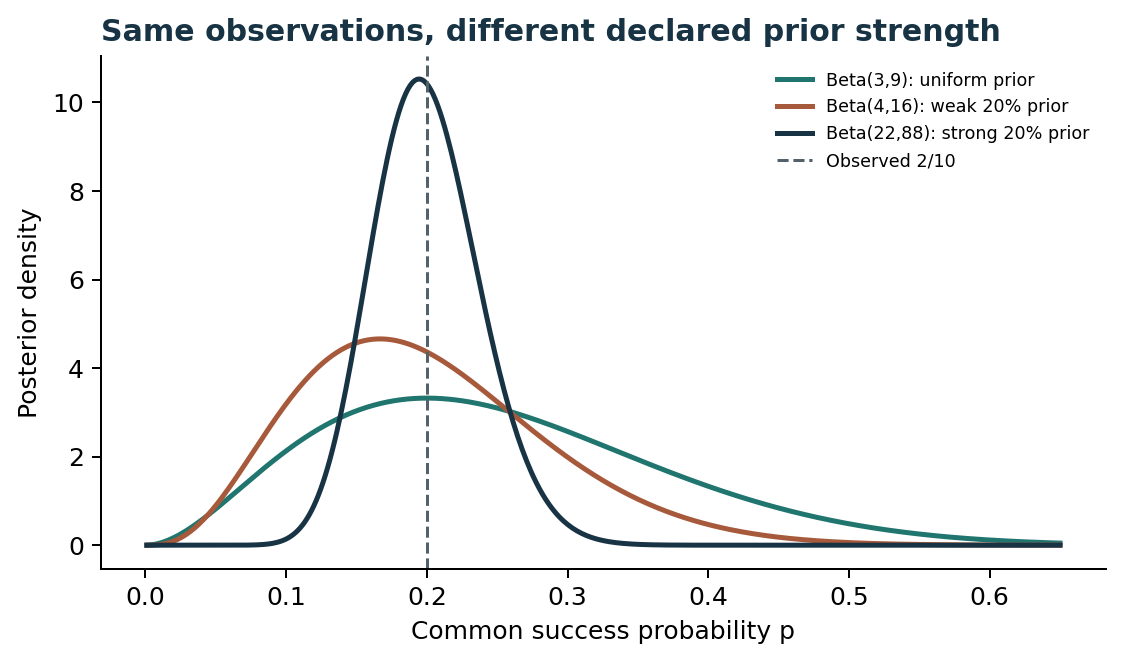
Enter a beta prior and binomial results. Watch how prior concentration and observed count combine under a stable independent-trial model.
Try three questions
- Which physical randomisation made each label rearrangement possible?
- Which entity would be independently resampled: row, customer, classroom, or device?
- Could the success probability change over time, making the beta likelihood misleading?
Download the executed Python lab · Read draft exercise solutions
Inspect the work.
Read the programs, run them in your own environment, and compare the results. The captured output records the chapter’s checked practical run; changing an input may change its answer.
Python resampling_bayes_lab.py
"""Chapter 10 constructed exact rearrangements, bootstrap and beta updates."""
from collections import Counter
from itertools import combinations, product
from math import comb, sqrt
from statistics import mean, median, pstdev, stdev

from scipy.stats import beta
from scipy.stats import betabinom

observed=(1,2,2,3,4,5,5,10)
stats=[]
for treated in combinations(range(8),4):
    s=sum(observed[i] for i in treated)
    stats.append(s/2-8)
counts=Counter(stats)
tail=sum(abs(x)>=4 for x in stats)
print(f"Permutation: assignments={len(stats)}, observed_difference=4.000000, two_sided_tail={tail}, exact_p={tail/len(stats):.6f}")
print("Permutation distribution:", ", ".join(f"{x:g}:{counts[x]}" for x in sorted(counts)))

source=(2,3,10)
boot=list(product(source,repeat=3))
means=[mean(x) for x in boot]
medians=Counter(median(x) for x in boot)
print(f"Bootstrap: ordered_resamples={len(boot)}, mean_of_means={mean(means):.6f}, mean_SE={pstdev(means):.6f}, original_s_over_root_n={stdev(source)/sqrt(3):.6f}, median_counts={dict(sorted(medians.items()))}")

for a,b in [(1,1),(2,8),(20,80)]:
    ap,bp=a+2,b+8
    lo,hi=beta.ppf([.025,.975],ap,bp)
    print(f"Beta: prior=({a},{b}), posterior=({ap},{bp}), mean={ap/(ap+bp):.6f}, 95%_equal_tail=[{lo:.6f},{hi:.6f}], P(p>.3)={beta.sf(.3,ap,bp):.6f}")
print("Sequential stable-p update: beta(1,1) + 2/10 + 8/10 = beta(11,11)")
predictive=[betabinom.pmf(k,10,3,9) for k in range(11)]
losses=[sum((s+10*max(k-s,0))*predictive[k] for k in range(11)) for s in range(11)]
print(f"Predictive next-ten: P(K>5)={sum(predictive[6:]):.6f}, stock_loss_0_to_10={[round(float(x),6) for x in losses]}, best_stock={min(range(11),key=lambda s:losses[s])}")

assert len(stats)==comb(8,4)==70 and tail==2
assert len(boot)==27 and abs(pstdev(means)-sqrt(38/9))<1e-12
assert medians=={2:7,3:13,10:7}
assert min(range(11),key=lambda s:losses[s])==5
Output Checked chapter run
Permutation: assignments=70, observed_difference=4.000000, two_sided_tail=2, exact_p=0.028571
Permutation distribution: -4:1, -3.5:1, -3:4, -2.5:5, -2:6, -1.5:6, -1:6, -0.5:4, 0:4, 0.5:4, 1:6, 1.5:6, 2:6, 2.5:5, 3:4, 3.5:1, 4:1
Bootstrap: ordered_resamples=27, mean_of_means=5.000000, mean_SE=2.054805, original_s_over_root_n=2.516611, median_counts={2: 7, 3: 13, 10: 7}
Beta: prior=(1,1), posterior=(3,9), mean=0.250000, 95%_equal_tail=[0.060218,0.517756], P(p>.3)=0.312740
Beta: prior=(2,8), posterior=(4,16), mean=0.200000, 95%_equal_tail=[0.060525,0.395785], P(p>.3)=0.133171
Beta: prior=(20,80), posterior=(22,88), mean=0.200000, 95%_equal_tail=[0.131024,0.279298], P(p>.3)=0.007755
Sequential stable-p update: beta(1,1) + 2/10 + 8/10 = beta(11,11)
Predictive next-ten: P(K>5)=0.063467, stock_loss_0_to_10=[25.0, 17.240602, 11.548872, 8.04644, 6.368421, 5.967492, 6.332817, 7.091093, 8.017776, 9.001871, 10.0], best_stock=5